Here is a list of (real!) data for globular clusters.The data give
We are going to use this data to learn about the distance to the galactic center, and the rotation speed of the Milky Way.
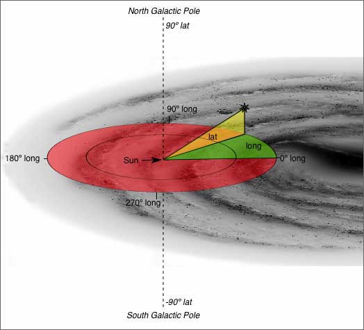
- the angular coordinates of each cluster in galactic coordinates (l,b). Note that these coordinates are different from the galactic coordinates discussed in class (yep, ain't life difficult?) - those coordinates (r, theta, z) measured position with respect to the center of the Galaxy, while these coordinates (l,b) are the observed angular position of the globular cluster, as viewed from the Sun (i.e., our viewing position). Here's an image showing the coordinate system. So l measures angle in the sky, with l=0o defined as pointing towards the Galactic Center, and l=90o pointing in the direction of the Galaxy's rotation. b measures angle above or below the plane of the Milky Way. If a cluster has coordinate (0o,20o), it would be viewed 20 degrees above the disk plane, in the direction of the Galactic Center. Got it?
- the distance from the Sun, R, in kiloparsecs
- the metallicity of the globular cluster, [Fe/H]. (Note: if [Fe/H] = 999, that means there is no measurement.)
- the observed radial velocity of the cluster, Vr, in km/s. (Note: if Vr = 999, that means there is no measurement.)
First, transform the observed data (l, b, R) into cartesian coordinates (X,Y,Z). +X should point towards the galactic center (l=0o), +Y should point in the direction of rotation (l=90o), and +Z should point above the plane (positive b). Defined this way, we have
- X=Rcos(l)cos(b)
- Y=Rsin(l)cos(b)
- Z=Rsin(b)
Coding alert: Be careful with trig functions when coding! numpy trig functions assume angles are given in radians, not degrees. But the data file lists angles in degrees, so you must convert. So Z=R*np.sin(b) would be incorrect, but Z=R*np.sin(np.radians(b)) will work.
Calculate and plot the X,Y,Z positions to get a feel for the distribution of globular clusters in the Galaxy. Plot the X-Y and X-Z projections so that you can see how things are distributed along each axis.
- Make X-Y and X-Z plots for the metal-poor globular clusters with [Fe/H] < -0.8
- Make the same plot for the metal-rich globular clusters with [Fe/H] > -0.8
- Note: Be careful not to include clusters which do not have measured [Fe/H]! So make sure to "filter" your data. Try something like this:
MR = (feh>-0.8) & (feh!=999) # define which clusters are metal rich
plt.scatter(x[MR],y[MR]) # only plot metal rich clusters
- Explain how the two distributions are different.
Coding alert: Make sure your plots have the same XYZ range, and that a circle would be a circle on your plot! Otherwise you won't be able to compare the shape and extent of the two distributions. Two tips for making this plot:
- Set the x and y limits on your plot by hand, rather than letting python autoscale the plot.
- Tell python you want equal axis ratio on your plots. Say plt.axis('equal'), or if you are using subplots, say <subplot_name>.set_aspect('equal').
Now, in the 1910s, Harlow Shapley derived the distance to the Galactic Center by using the positions of the globular clusters. Now it's your turn:Finally, we can use the observed velocities of the globular clusters to get the rotation speed of the Galaxy.
- What is the (X,Y,Z) center of the metal-poor globular cluster system? How far, then, is the Galactic Center?
- What is the (X,Y,Z) center of the metal-rich globular cluster system? How far, then, is the Galactic Center?
- Which of these two measurements do you feel is more accurate? Why?
So we should be able to fit a sine function to the data: Vr = -Vc,proj sin(l). Once you have solved for Vc,proj, remember we have to deproject this value to get the true rotation speed. Since Vc,proj = Vc<cos(b)>, averaging over all b's, we have Vc,proj = (2/pi)Vc. So to correct for projection, Vc = (pi/2)Vc,proj.
- Plot Vr (on the y-axis) against l (on the x-axis). Only use the metal-poor globular clusters for this exercise. Why? You should see a lot of dispersion, but a hint of a sinusoidal trend. At l=90o the radial velocities are more negative, at l=270o they are more positive. This is because the globular cluster system isn't rotating. Remember that l=90o points along the direction of rotation; clusters along l=90o are in front of us and we are moving towards them, so they have a negative (approaching) radial velocity (and vice versa for the clusters at l=270o).
- Note: Make sure not to include clusters which have no measured Vr in your analysis! Use the filtering technique we talked about above.
- Fit this sine curve to the data, and derive Vc, the circular velocity of the Milky Way. How does your value compare to the "standard" value of 220 km/s?
Coding alert: remember you dont actually have to do a sine fit of Vr versus l which would be a complicated non-linear fit. Instead, fit Vr versus sin(l), which is a simple linear fit! (But remember to convert l to radians when using the sine function!)
Now, what is the velocity dispersion of the globular cluster system? That is, if the globular clusters weren't moving at all, the sine fit would work perfectly, and go through all the data points (projection effects aside). It clearly doesn't -- there is a lot of scatter around that line. That tells us that the clusters themselves are moving as well, but in a random sense, rather than as a rotating system. The scatter of the velocities around the sine fit gives us an estimate of how fast the clusters are moving in this random motion, which is referred to as their velocity dispersion.
You can estimate the scatter around a fit by calculating the the standard deviation of the residuals. In other words, for each data point, calculate the residual as residual = Vr - Vr,fit = Vr + Vc,proj sin(l), and then calculating the standard deviation of the residuals. Again you'll want to correct your scatter for projection effects, this time by multiplying your std deviation by root(3) since we're only seeing one of the three velocity components of each cluster's motion.
- From your plot and fit, estimate the velocity dispersion of the globular cluster system. Compare it to the rotation speed of the Milky Way's disk. They ought to be roughly similar -- why?
This dataset contains apparent magnitude (V), radial velocity (vrad), and absolute magnitudes (MV) for a sample of K giant stars along a line of sight at galactic latitude b ~ -90o (in other words looking directly out of the plane of the Milky Way's disk). We are going to use this dataset to measure the mass density of the Milky Way's disk in the solar neighborhood. Remember how we do this, by using the Oort limit, which means we need the velocity dispersion and scale height of the stars.Scale Height
Calculate the distance to each star from its apparent and absolute magnitude. Because these stars are all at b ~ -90o, their Z distance from the plane is pretty much given by the distance of the star, once we correct for the distance of the Sun from the galactic plane. Since the Sun is "above" the disk plane (at Z=+30 pc) and these stars are seen "below" the disk plane, their distance from the disk plane is simply given by Z = distance - 30 pc.Velocity DispersionThen find the number of stars (N) as a function of Z by making bins of, say, 200 pc size and counting the number of stars in each bin. Make a plot of ln(N) (y axis) vs Z (x axis) and find the scale height of the stars (how?). When fitting, remember to make smart choices about which bins to include in your fit; including all your bins is probably not a good choice!
Coding alert: First, take a look at the binning and fitting example code on the Python help page to figure out how to code up this exercise. Also, be careful with logs when coding. In numpy, np.log(x) means "natural log of x" and np.log10(x) means "base 10 log of x". Make sure you use the correct one when doing calculations! In this case we want the natural log, since we are plotting an exponential function.
Just like we said the distance was roughly the Z coordinate (once we corrected for the Sun's Z coordinate), we can also say the radial velocity is roughly the Z velocity once we correct for the Sun's Z velocity.The Oort limitFrom the distribution of velocities, calculate the Sun's Z velocity (how?). Then subtract that from all the velocities to get the Z velocity of each star. Then bin up the stars in a few bins of Z, calculate the dispersion of each of the bins (how?), and then make a plot of velocity dispersion as a function of Z height. How and why does it change with Z?
Given the scale height and velocity dispersion (which velocity dispersion do you use, and why?), estimate the mass density of the disk using the method shown in class. Describe sources of error and how they may have affected your result.